This example has been auto-generated from the examples/ folder at GitHub repository.
Conjugate-Computational Variational Message Passing (CVI)
# Activate local environment, see `Project.toml`
import Pkg; Pkg.activate(".."); Pkg.instantiate();
using RxInfer, Random, LinearAlgebra, Plots, Optimisers, Plots, StableRNGs, SpecialFunctionsIn this notebook, the usage of Conjugate-NonConjugate Variational Inference (CVI) will be described. The implementation of CVI follows the paper Probabilistic programming with stochastic variational message passing.
This notebook will first describe an example in which CVI is used, then it discusses several limitations, followed by an explanation on how to extend upon CVI.
An example: nonlinear dynamical system
A group of researchers is performing a tracking experiment on some moving object along a 1-dimensional trajectory. The object is moving at a constant velocity, meaning that its position increases constantly over time. However, the researchers do not have access to the absolute position $z_t$ at time $t$. Instead they have access to the observed squared distance $y_t$ between the object and some reference point $s$. Because of budget cuts, the servo moving the object and the measurement devices are quite outdated and therefore lead to noisy measurements:
# data generating process
nr_observations = 50
reference_point = 53
hidden_location = collect(1:nr_observations) + rand(StableRNG(124), NormalMeanVariance(0.0, sqrt(5)), nr_observations)
measurements = (hidden_location .- reference_point).^2 + rand(MersenneTwister(124), NormalMeanVariance(0.0, 5), nr_observations);
# plot hidden location and reference frame
p1 = plot(1:nr_observations, hidden_location, linewidth=3, legend=:topleft, label="hidden location")
hline!([reference_point], linewidth=3, label="reference point")
xlabel!("time [sec]"), ylabel!("location [cm]")
# plot measurements
p2 = scatter(1:nr_observations, measurements, linewidth=3, label="measurements")
xlabel!("time [sec]"), ylabel!("squared distance [cm2]")
plot(p1, p2, size=(1200, 500))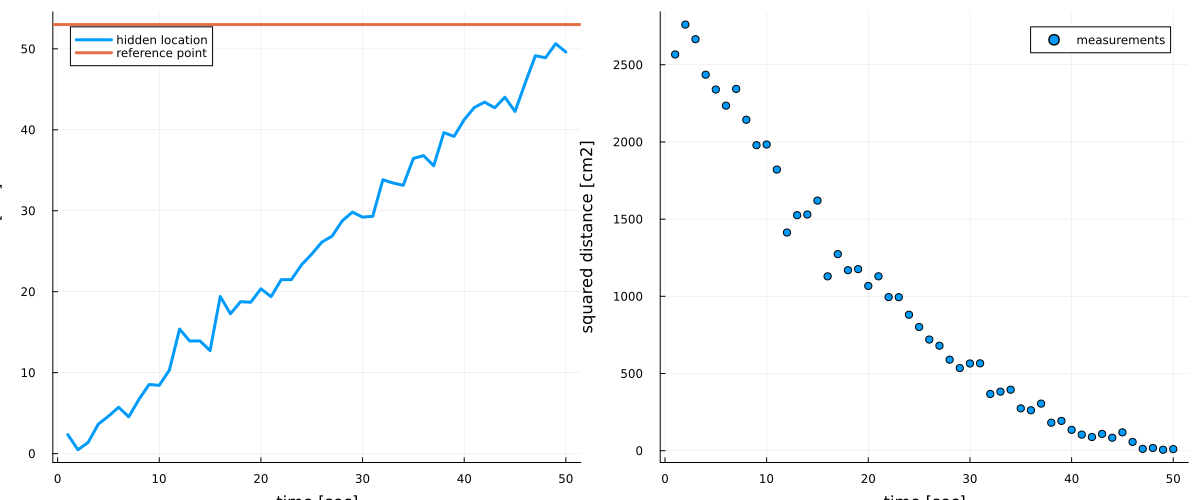
The researchers are interested in quantifying this noise and in tracking the unobserved location of the object. As a result of this uncertainty, the researchers employ a probabilistic modeling approach. They formulate the probabilistic model
\[\begin{aligned} p(\tau) & = \Gamma(\tau \mid \alpha_{\tau}, \beta_{\tau}),\\ p(\gamma) & = \Gamma(\gamma \mid \alpha_{\gamma}, \beta_{\gamma}),\\ p(z_t \mid z_{t - 1}, \tau) & = \mathcal{N}(z_t \mid z_{t - 1} + 1, \tau^{-1}),\\ p(y_t \mid z_t, \gamma) & = \mathcal{N}(y_t \mid (z_t - s)^2, \gamma^{-1}), \end{aligned}\]
where the researchers put priors on the process and measurement noise parameters, $\tau$ and $\gamma$, respectively. They do this, because they do not know the accuracy of their devices.
The researchers have recently heard of this cool probabilistic programming package RxInfer.jl. They decided to give it a try and create the above model as follows:
function compute_squared_distance(z)
    (z - reference_point)^2
end;
@model function measurement_model(y)
# set priors on precision parameters
τ ~ Gamma(shape = 0.01, rate = 0.01)
γ ~ Gamma(shape = 0.01, rate = 0.01)
# specify estimate of initial location
z[1] ~ Normal(mean = 0, precision = τ)
y[1] ~ Normal(mean = compute_squared_distance(z[1]), precision = γ)
# loop over observations
for t in 2:length(y)
# specify state transition model
z[t] ~ Normal(mean = z[t-1] + 1, precision = τ)
# specify non-linear observation model
y[t] ~ Normal(mean = compute_squared_distance(z[t]), precision = γ)
end
endBut here is the problem, our compute_squared_distance function is already compelx enough such that the exact Bayesian inference is intractable in this model. But the researchers knew that the RxInfer.jl supports a various collection of approximation methods for exactly such cases. One of these approximations is called CVI. CVI allows us to perform probabilistic inference around the non-linear measurement function. In general, for any (non-)linear relationship y = f(x1, x2, ..., xN) CVI can be employed, by specifying the function f and by adding this relationship inside the @model macro as y ~ f(x1, x2, ...,xN). The @model macro will generate a factor node with node function p(y | x1, x2, ..., xN) = δ(y - f(x1, x2, ...,xN)).
The use of this non-linearity requires us to specify that we would like to use CVI. This can be done by specifying the metadata using the @meta macro as:
@meta function measurement_meta(rng, nr_samples, nr_iterations, optimizer)
    compute_squared_distance() -> CVI(rng, nr_samples, nr_iterations, optimizer)
end;
In general, for any (non-)linear function f(), CVI can be enabled with the @meta macro as:
@meta function model_meta(...)
    f() -> CVI(args...)
end
See ?CVI for more information about the args....
In our model, the z variables are connected to the non-linear node function. So in order to run probabilstic inference with CVI we need to enforce a constraint on the joint posterior distribution. Specifically, we need to create a factorization in which the variables that are directly connected to non-linearities are assumed to be independent from the rest of the variables.
In the above example, we will assume the following posterior factorization:
@constraints function measurement_constraints()
    q(z, τ, γ) = q(z)q(τ)q(γ)
end;
This constraint can be explained by the set of two constraints, one for getting CVI to run, and one for assuming a mean-field factorization around the normal node as
@constraints function posterior_constraints() begin
    q(z, γ) = q(z)q(γ) # CVI
    q(z, τ) = q(z)q(τ) # the mean-field assumption around normal node
end
Because the engineers are using RxInfer.jl, they can automate the inference procedure. They track the inference performance using the Bethe free energy.
initialization = @initialization begin
    μ(z) = NormalMeanVariance(0, 5)
    q(z) = NormalMeanVariance(0, 5)
    q(τ) = GammaShapeRate(1e-12, 1e-3)
    q(γ) = GammaShapeRate(1e-12, 1e-3)
end

results = infer(
    model = measurement_model(),
    data = (y = measurements,),
    iterations = 50,
    free_energy = true,
    returnvars = (z = KeepLast(),),
    constraints = measurement_constraints(),
    meta = measurement_meta(StableRNG(42), 1000, 1000, Optimisers.Descent(0.001)),
    initialization = initialization
)
Inference results:
Posteriors | available for (z)
Free Energy: | Real[506.207, 327.398, 325.066, 320.864, 315.809, 312.
717, 310.775, 309.344, 308.486, 308.456 … 306.705, 306.266, 306.172, 306.
587, 306.621, 306.501, 306.382, 306.512, 306.659, 306.485]# plot estimates for location
p1 = plot(collect(1:nr_observations), hidden_location, label = "hidden location", legend=:topleft, linewidth=3, color = :red)
plot!(map(mean, results.posteriors[:z]), label = "estimated location (±2σ)", ribbon = map(x -> 2*std(x), results.posteriors[:z]), fillalpha=0.5, linewidth=3, color = :orange)
xlabel!("time [sec]"), ylabel!("location [cm]")
# plot Bethe free energy
p2 = plot(results.free_energy, linewidth=3, label = "")
xlabel!("iteration"), ylabel!("Bethe free energy [nats]")
plot(p1, p2, size = (1200, 500))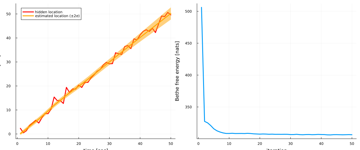
Requirements
There are several main requirements for the CVI procedure to satisfy:
- The
outinterface of the non-linearity must be independently factorized with respect to other variables in the model. - The messages on input interfaces (
x1, x2, ..., xN) are required to be from the exponential family of distributions.
In RxInfer, you can satisfy the first requirement by using appropriate factor nodes (Normal, Gamma, Bernoulli, etc) and second requirement by specifying the @constraints macro. In general you can specify this procedure as
@model function model(...)
    ...
    y ~ f(x1, x2, ..., xN)
    ... ~ Node2(z1,..., y, zM) # some node that is using the out interface of the non-linearity
    ...
end

@constraints function constraints_meta() begin
    q(y, z1, ..., zn) = q(y)q(z1,...,zM)
    ...
end;

@meta function model_meta(...)
    f() -> CVI(rng, nr_samples, nr_iterations, optimizer))
end
Note that not all exponential family distributions are implemented.
Extensions
Using a custom optimizer
CVI only supports Optimisers optimizers out of the box.
Below an explanation on how to extend to it to a custom optimizer.
Suppose we have CustomDescent structure which we want to use inside CVI for optimization.
To do so, we need to implement ReactiveMP.cvi_update!(opt::CustomDescent, λ, ∇).
ReactiveMP.cvi_update! incapsulates the gradient step:
optis used to select your optimizer structureλis the current value∇is a gradient value computed insideCVI.
struct CustomDescent
    learning_rate::Float64
end

# Must return an optimizer and its initial state
function ReactiveMP.cvi_setup(opt::CustomDescent, q)
     return (opt, nothing)
end

# Must return an updated (opt, state) and an updated λ (can use new_λ for inplace operation)
function ReactiveMP.cvi_update!(opt_and_state::Tuple{CustomDescent, Nothing}, new_λ, λ, ∇)
    opt, _ = opt_and_state
    λ̂ = vec(λ) - (opt.learning_rate .* vec(∇))
    copyto!(new_λ, λ̂)
    return opt_and_state, new_λ
end
Let's try to apply it to a model: $\begin{aligned} p(x) & = \mathcal{N}(0, 1),\\ p(y_{i}\mid x) & = \mathcal{N}(y_i \mid x^2, 1),\\ \end{aligned}$
Let's generate some synthetic data for the model
# generate data
y = rand(StableRNG(123), NormalMeanVariance(19^2, 10), 1000)
histogram(y)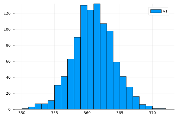
Again we can create the corresponding model as:
# specify non-linearity
f(x) = x ^ 2

# specify model
@model function normal_square_model(y)
    # describe prior on latent state, we set an arbitrary prior
    # in a positive domain
    x ~ Normal(mean = 5, precision = 1e-3)
    # transform latent state
    mean := f(x)
    # observation model
    y .~ Normal(mean = mean, precision = 0.1)
end

# specify meta
@meta function normal_square_meta(rng, nr_samples, nr_iterations, optimizer)
    f() ->  CVI(rng, nr_samples, nr_iterations, optimizer)
end
normal_square_meta (generic function with 1 method)We will use the inference function from ReactiveMP to run inference, where we provide an instance of the CustomDescent structure in our meta macro function:
res = infer(
    model = normal_square_model(),
    data = (y = y,),
    iterations = 5,
    free_energy = true,
    meta = normal_square_meta(StableRNG(123), 1000, 1000, CustomDescent(0.001)),
    free_energy_diagnostics = nothing
)

mean(res.posteriors[:x][end])18.992828536095285The mean inferred value of x is indeed close to 19, which was used to generate the data. Inference is working!
p1 = plot(mean.(res.posteriors[:x]), ribbon = 3std.(res.posteriors[:x]), label = "Posterior estimation", ylim = (0, 40))
p2 = plot(res.free_energy, label = "Bethe Free Energy")

plot(p1, p2, layout = @layout([ a b ]))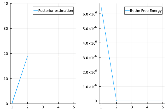
Note: $x^2$ can not be inverted; the sign information can be lost: -19 and 19 are both equally good solutions.